Labelling data and comparing classification algorithms#
import matplotlib.pyplot as plt
import numpy as np
import pandas as pd
from sklearn import model_selection, preprocessing
from sklearn.discriminant_analysis import LinearDiscriminantAnalysis
from sklearn.ensemble import RandomForestClassifier
from sklearn.linear_model import LogisticRegression
from sklearn.metrics import (
    accuracy_score,
    classification_report,
    confusion_matrix,
)
from sklearn.naive_bayes import GaussianNB
from sklearn.neighbors import KNeighborsClassifier
from sklearn.neural_network import MLPClassifier
from sklearn.tree import DecisionTreeClassifier
# import data
df = pd.read_csv("data/SCADA_downtime_merged.csv", skip_blank_lines=True)
# list of turbines to plot
list1 = [1]
# list1 = list(df['turbine_id'].unique())
# sort turbines in ascending order
# list1 = sorted(list1, key=int)
# list of categories to plot
list2 = [10, 11]
# list2 = list(df['TurbineCategory_id'].unique())
# list2 = [g for g in list2 if g >= 0]
# sort categories in ascending order
# list2 = sorted(list2, key=int)
# categories to remove from plot
# list2 = [m for m in list2 if m not in (1, 12, 13, 14, 15, 17, 21, 22)]
for x in list1:
# filter only data for turbine x
dfx = df[(df["turbine_id"] == x)].copy()
for y in list2:
# copying fault to new column (mins) (fault when turbine category id
# is y)
def f(c):
if c["TurbineCategory_id"] == y:
return 0
else:
return 1
dfx["mins"] = dfx.apply(f, axis=1)
# sort values by timestamp in descending order
dfx = dfx.sort_values(by="timestamp", ascending=False)
# reset index
dfx.reset_index(drop=True, inplace=True)
# assigning value to first cell if it's not 0
if dfx.loc[0, "mins"] == 0:
dfx.set_value(0, "mins", 0)
else:
dfx.set_value(0, "mins", 999999999)
# using previous value's row to evaluate time
for i, e in enumerate(dfx["mins"]):
if e == 1:
dfx.at[i, "mins"] = dfx.at[i - 1, "mins"] + 10
# sort in ascending order
dfx = dfx.sort_values(by="timestamp")
# reset index
dfx.reset_index(drop=True, inplace=True)
# convert to hours and round to nearest hour
dfx["hours"] = dfx["mins"].astype(np.int64)
dfx["hours"] = dfx["hours"] / 60
dfx["hours"] = round(dfx["hours"]).astype(np.int64)
# > 48 hours - label as normal (9999)
def f1(c):
if c["hours"] > 48:
return 9999
else:
return c["hours"]
dfx["hours"] = dfx.apply(f1, axis=1)
# filter out curtailment - curtailed when turbine is pitching outside
# 0deg <= normal <= 3.5deg
def f2(c):
if (
0 <= c["pitch"] <= 3.5
or c["hours"] != 9999
or (
(c["pitch"] > 3.5 or c["pitch"] < 0)
and (
c["ap_av"] <= (0.1 * dfx["ap_av"].max())
or c["ap_av"] >= (0.9 * dfx["ap_av"].max())
)
)
):
return "normal"
else:
return "curtailed"
dfx["curtailment"] = dfx.apply(f2, axis=1)
# filter unusual readings, i.e. for normal operation, power <= 0 in
# operating wind speeds, power > 100 before cut-in, runtime < 600 and
# other downtime categories
def f3(c):
if c["hours"] == 9999 and (
(
3 < c["ws_av"] < 25
and (
c["ap_av"] <= 0
or c["runtime"] < 600
or c["EnvironmentalCategory_id"] > 1
or c["GridCategory_id"] > 1
or c["InfrastructureCategory_id"] > 1
or c["AvailabilityCategory_id"] == 2
or 12 <= c["TurbineCategory_id"] <= 15
or 21 <= c["TurbineCategory_id"] <= 22
)
)
or (c["ws_av"] < 3 and c["ap_av"] > 100)
):
# remove unusual readings, i.e., zero power at operating wind
# speeds, power > 0 before cut-in ...
return "unusual"
else:
return "normal"
dfx["unusual"] = dfx.apply(f3, axis=1)
# round to 6 hour intervals
def f4(c):
if 1 <= c["hours"] <= 6:
return 6
elif 7 <= c["hours"] <= 12:
return 12
elif 13 <= c["hours"] <= 18:
return 18
elif 19 <= c["hours"] <= 24:
return 24
elif 25 <= c["hours"] <= 30:
return 30
elif 31 <= c["hours"] <= 36:
return 36
elif 37 <= c["hours"] <= 42:
return 42
elif 43 <= c["hours"] <= 48:
return 48
else:
return c["hours"]
dfx["hours6"] = dfx.apply(f4, axis=1)
# change label for unusual and curtailed data
def f5(c):
if c["unusual"] == "unusual" or c["curtailment"] == "curtailed":
return -9999
else:
return c["hours6"]
dfx["hours_%s" % y] = dfx.apply(f5, axis=1)
# drop unnecessary columns
dfx = dfx.drop("hours6", axis=1)
dfx = dfx.drop("hours", axis=1)
dfx = dfx.drop("mins", axis=1)
dfx = dfx.drop("curtailment", axis=1)
dfx = dfx.drop("unusual", axis=1)
df2 = dfx[
[
"ap_av",
"ws_av",
"wd_av",
"pitch",
"ap_max",
"ap_dev",
"reactive_power",
"rs_av",
"gen_sp",
"nac_pos",
"hours_11",
]
].copy()
df2 = df2.dropna()
# splitting data set
features = [
"ap_av",
"ws_av",
"wd_av",
"pitch",
"ap_max",
"ap_dev",
"reactive_power",
"rs_av",
"gen_sp",
"nac_pos",
]
X = df2[features]
Y = df2["hours_11"]
Xn = preprocessing.normalize(X)
validation_size = 0.20
seed = 7
X_train, X_validation, Y_train, Y_validation = (
model_selection.train_test_split(
Xn, Y, test_size=validation_size, random_state=seed
)
)
models = []
models.append(("LR", LogisticRegression(class_weight="balanced")))
models.append(("LDA", LinearDiscriminantAnalysis()))
models.append(("KNN5", KNeighborsClassifier()))
models.append(("KNN15", KNeighborsClassifier(n_neighbors=15)))
models.append(("DT", DecisionTreeClassifier(class_weight="balanced")))
models.append(("RF", RandomForestClassifier(class_weight="balanced")))
models.append(("NB", GaussianNB()))
models.append(("MLP", MLPClassifier()))
# evaluate each model in turn
results = []
names = []
msg1 = "Results for Turbine %s" % x + " with Turbine Category %s" % y
print(msg1)
for name, model in models:
kfold = model_selection.KFold(n_splits=10, random_state=seed)
cv_results = model_selection.cross_val_score(
model, X_train, Y_train, cv=kfold, scoring="accuracy"
)
results.append(cv_results)
names.append(name)
msg = "{}: {:f} ({:f})".format(
name, cv_results.mean(), cv_results.std()
)
print(msg)
# compare algorithms
fig = plt.figure()
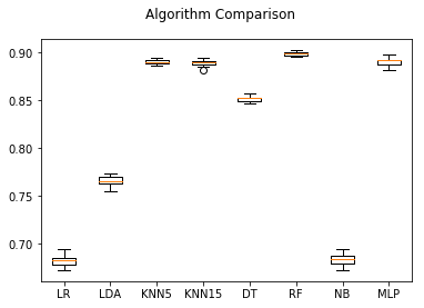
fig.suptitle("Algorithm Comparison")
ax = fig.add_subplot(111)
plt.boxplot(results)
ax.set_xticklabels(names)
plt.show()
Results for Turbine 1 with Turbine Category 11
LR: 0.682084 (0.006069)
LDA: 0.765452 (0.005270)
KNN5: 0.889947 (0.002742)
KNN15: 0.888914 (0.003590)
DT: 0.851390 (0.003076)
RF: 0.899010 (0.002075)
NB: 0.683200 (0.006298)
MLP: 0.890631 (0.004285)
clf2 = RandomForestClassifier(class_weight="balanced")
clf2.fit(X_train, Y_train)
predictions2 = clf2.predict(X_validation)
print(accuracy_score(Y_validation, predictions2))
print(confusion_matrix(Y_validation, predictions2))
print(classification_report(Y_validation, predictions2))
0.903127204326
[[  369     5     4     1     1     0     0     0     3    37]
 [    3    57    13     1     1     0     2     0     0   202]
 [    5     9    60     2     0     0     0     0     1   160]
 [    1     7     6    50     3     0     0     4     0   140]
 [    0     1     4     3    22     0     1     1     2   124]
 [    0     0     3     0     5    33     2     2     2    98]
 [    0     1     0     0     2     3    31     1     0   124]
 [    4     1     0     3     0     1     1    19     3   114]
 [    1     0     3     1     0     0     1     3    22   107]
 [    4    22   356     9     6     6     7     3     2 14701]]
             precision    recall  f1-score   support

          0       0.95      0.88      0.91       420
          6       0.55      0.20      0.30       279
         12       0.13      0.25      0.17       237
         18       0.71      0.24      0.36       211
         24       0.55      0.14      0.22       158
         30       0.77      0.23      0.35       145
         36       0.69      0.19      0.30       162
         42       0.58      0.13      0.21       146
         48       0.63      0.16      0.25       138
       9999       0.93      0.97      0.95     15116

avg / total       0.90      0.90      0.89     17012
clf = KNeighborsClassifier()
clf.fit(X_train, Y_train)
predictions = clf.predict(X_validation)
print(accuracy_score(Y_validation, predictions))
print(confusion_matrix(Y_validation, predictions))
print(classification_report(Y_validation, predictions))
0.913825534917
[[  361     6     2     3     0     0     1     0     0    47]
 [    6    28     7     3     5     1     2     1     0   226]
 [    7     9    40     4     3     0     0     0     0   174]
 [    3     9    11    40     3     1     0     2     1   141]
 [    1     0     0     7    15     3     0     2     0   130]
 [    3     3     2     1     3    28     3     2     1    99]
 [    2     2     0     2     1     3    30     1     1   120]
 [    4     0     2     6     0     1     4    23     3   103]
 [    2     0     2     1     1     0     1     1    19   111]
 [   15    36    19    21    13    15    16    11     8 14962]]
             precision    recall  f1-score   support

          0       0.89      0.86      0.88       420
          6       0.30      0.10      0.15       279
         12       0.47      0.17      0.25       237
         18       0.45      0.19      0.27       211
         24       0.34      0.09      0.15       158
         30       0.54      0.19      0.28       145
         36       0.53      0.19      0.27       162
         42       0.53      0.16      0.24       146
         48       0.58      0.14      0.22       138
       9999       0.93      0.99      0.96     15116

avg / total       0.89      0.91      0.89     17012
print(dfx.groupby("hours6").size())
hours6
0         2204
6         1719
12        1289
18        1070
24         913
30         787
36         756
42         727
48         684
9999    121179
dtype: int64