Comparing random forest classifier performance#

import matplotlib.pyplot as plt
import numpy as np
import pandas as pd
from sklearn import preprocessing
from sklearn.ensemble import RandomForestClassifier
from sklearn.model_selection import TimeSeriesSplit
# import data
df = pd.read_csv("data/SCADA_downtime_merged.csv", skip_blank_lines=True)
# list of turbines to plot
list1 = list(df["turbine_id"].unique())
# sort turbines in ascending order
list1 = sorted(list1, key=int)
# list of categories
list2 = list(df["TurbineCategory_id"].unique())
# remove NaN from list
list2 = [g for g in list2 if g >= 0]
# sort categories in ascending order
list2 = sorted(list2, key=int)
# categories to remove
list2 = [m for m in list2 if m not in (1, 12, 13, 14, 15, 17, 21, 22)]
# empty list to hold optimal n values for all turbines
num = []
# empty list to hold minimum error readings for all turbines
err = []
# filter only data for turbine x
for x in list1:
    dfx = df[(df["turbine_id"] == x)].copy()

    # copying fault to new column (mins) (fault when turbine category id is y)
    for y in list2:

        def f(c):
            if c["TurbineCategory_id"] == y:
                return 0
            else:
                return 1

        dfx["mins"] = dfx.apply(f, axis=1)

        # sort values by timestamp in descending order
        dfx = dfx.sort_values(by="timestamp", ascending=False)
        # reset index
        dfx.reset_index(drop=True, inplace=True)

        # assigning value to first cell if it's not 0 with a large number
        if dfx.loc[0, "mins"] == 0:
            dfx.set_value(0, "mins", 0)
        else:
            # to allow the following loop to work
            dfx.set_value(0, "mins", 999999999)

        # using previous value's row to evaluate time
        for i, e in enumerate(dfx["mins"]):
            if e == 1:
                dfx.at[i, "mins"] = dfx.at[i - 1, "mins"] + 10

        # sort in ascending order
        dfx = dfx.sort_values(by="timestamp")
        # reset index
        dfx.reset_index(drop=True, inplace=True)
        # convert to hours, then round to nearest hour
        dfx["hours"] = dfx["mins"].astype(np.int64)
        dfx["hours"] = dfx["hours"] / 60
        # round to integer
        dfx["hours"] = round(dfx["hours"]).astype(np.int64)

        # > 48 hours - label as normal (999)
        def f1(c):
            if c["hours"] > 48:
                return 999
            else:
                return c["hours"]

        dfx["hours"] = dfx.apply(f1, axis=1)

        # filter out curtailment - curtailed when turbine is pitching outside
        # 0deg <= normal <= 3.5deg
        def f2(c):
            if (
                0 <= c["pitch"] <= 3.5
                or c["hours"] != 999
                or (
                    (c["pitch"] > 3.5 or c["pitch"] < 0)
                    and (
                        c["ap_av"] <= (0.1 * dfx["ap_av"].max())
                        or c["ap_av"] >= (0.9 * dfx["ap_av"].max())
                    )
                )
            ):
                return "normal"
            else:
                return "curtailed"

        dfx["curtailment"] = dfx.apply(f2, axis=1)

        # filter unusual readings, i.e., for normal operation, power <= 0 in
        # operating wind speeds, power > 100 ...
        def f3(c):
            # before cut-in, runtime < 600 and other downtime categories
            if c["hours"] == 999 and (
                (
                    3 < c["ws_av"] < 25
                    and (
                        c["ap_av"] <= 0
                        or c["runtime"] < 600
                        or c["EnvironmentalCategory_id"] > 1
                        or c["GridCategory_id"] > 1
                        or c["InfrastructureCategory_id"] > 1
                        or c["AvailabilityCategory_id"] == 2
                        or 12 <= c["TurbineCategory_id"] <= 15
                        or 21 <= c["TurbineCategory_id"] <= 22
                    )
                )
                or (c["ws_av"] < 3 and c["ap_av"] > 100)
            ):
                return "unusual"
            else:
                return "normal"

        dfx["unusual"] = dfx.apply(f3, axis=1)

        # round to 6 hour intervals to reduce number of classes
        def f4(c):
            if 1 <= c["hours"] <= 6:
                return 6
            elif 7 <= c["hours"] <= 12:
                return 12
            elif 13 <= c["hours"] <= 18:
                return 18
            elif 19 <= c["hours"] <= 24:
                return 24
            elif 25 <= c["hours"] <= 30:
                return 30
            elif 31 <= c["hours"] <= 36:
                return 36
            elif 37 <= c["hours"] <= 42:
                return 42
            elif 43 <= c["hours"] <= 48:
                return 48
            else:
                return c["hours"]

        dfx["hours6"] = dfx.apply(f4, axis=1)

        # change label for unusual and curtailed data (9999), if originally
        # labelled as normal
        def f5(c):
            if c["unusual"] == "unusual" or c["curtailment"] == "curtailed":
                return 9999
            else:
                return c["hours6"]

        # apply to new column specific to each fault
        dfx["hours_%s" % y] = dfx.apply(f5, axis=1)

        # drop unnecessary columns
        dfx = dfx.drop("hours6", axis=1)
        dfx = dfx.drop("hours", axis=1)
        dfx = dfx.drop("mins", axis=1)
        dfx = dfx.drop("curtailment", axis=1)
        dfx = dfx.drop("unusual", axis=1)

    features = [
        "ap_av",
        "ws_av",
        "wd_av",
        "pitch",
        "ap_max",
        "ap_dev",
        "reactive_power",
        "rs_av",
        "gen_sp",
        "nac_pos",
    ]
    # separate features from classes for classification
    classes = [col for col in dfx.columns if "hours" in col]
    # list of columns to copy into new df
    list3 = features + classes + ["timestamp"]
    df2 = dfx[list3].copy()
    # drop NaNs
    df2 = df2.dropna()
    X = df2[features]
    # normalise features to values b/w 0 and 1
    X = preprocessing.normalize(X)
    Y = df2[classes]
    # convert from pd dataframe to np array
    Y = Y.as_matrix()

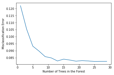
    # evaluating optimal number of trees
    # creating odd list of n
    myList = list(range(1, 30))
    # subsetting just the odd ones
    estimators = list(filter(lambda x: x % 2 != 0, myList))
    # empty list that will hold average cross validation scores for each n
    scores = []
    # cross validation using time series split
    tscv = TimeSeriesSplit(n_splits=5)

    # looping for each value of n and defining random forest classifier
    for n in estimators:
        rf = RandomForestClassifier(
            criterion="entropy",
            class_weight="balanced_subsample",
            random_state=42,
            n_estimators=n,
            n_jobs=-1,
        )
        # empty list to hold score for each cross validation fold
        p1 = []
        # looping for each cross validation fold
        for train_index, test_index in tscv.split(X):
            # split train and test sets
            X_train, X_test = X[train_index], X[test_index]
            Y_train, Y_test = Y[train_index], Y[test_index]
            # fit to classifier and predict
            rf1 = rf.fit(X_train, Y_train)
            pred = rf1.predict(X_test)
            # accuracy score
            p2 = (
                np.sum(np.equal(np.array(Y_test), pred))
                / np.array(Y_test).size
            )
            # add to list
            p1.append(p2)
        # average score across all cross validation folds
        p = sum(p1) / len(p1)
        scores.append(p)
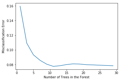
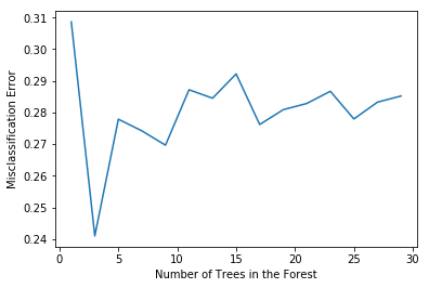
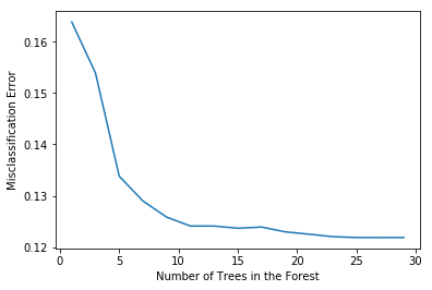
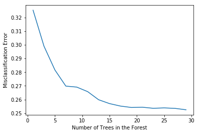
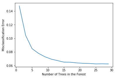
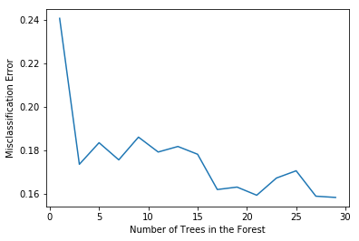
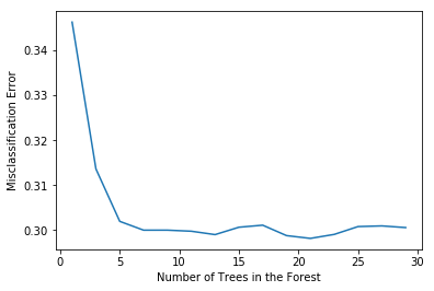
    # changing to misclassification error
    MSE = [1 - x for x in scores]
    # determining best n
    optimal_n = estimators[MSE.index(min(MSE))]
    num.append(optimal_n)
    err.append(min(MSE))

    print(
        "The optimal number of trees in the forest for turbine %s" % x
        + " is %d" % optimal_n
    )
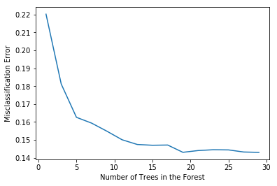
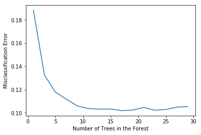
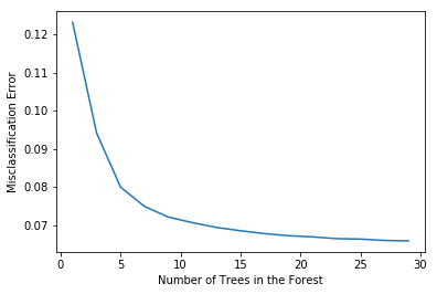
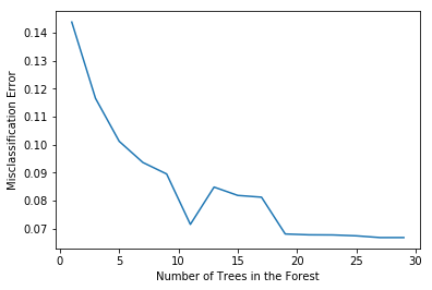
    # plot misclassification error vs n
    plt.plot(estimators, MSE)
    plt.xlabel("Number of Trees in the Forest")
    plt.ylabel("Misclassification Error")
    plt.show()
The optimal number of trees in the forest for turbine 1 is 29
../../_images/b6ff6d01135e244401fd40af00eea8c7798d95198beb119741f858054be04859.png
The optimal number of trees in the forest for turbine 2 is 17
../../_images/2686168cd6b2a4029eda39226e45635315bd94b580f8be338c012b41fd9e4973.png
The optimal number of trees in the forest for turbine 3 is 29
../../_images/40dc77bf00315d33ab0f69032d5e7b6925f4f86bdda0223b527ccd911210d335.png
The optimal number of trees in the forest for turbine 4 is 27
../../_images/b5f63347dc5701cda698b7bbad249c7a35629c60d70b7d0ee998123588095821.png
The optimal number of trees in the forest for turbine 5 is 11
../../_images/3da786bd16635f4928a5eb6a0e7605ffe3400a89dae90865f5c31a0bcca9cd20.png
The optimal number of trees in the forest for turbine 6 is 3
../../_images/200c414f84b4e8cc3e5abcebb740ee8a764edfb69f2951cf75f439c31a91b7c0.png
The optimal number of trees in the forest for turbine 7 is 27
../../_images/b97a95ce1b81ca659995e082e834c0c062b3aff98163cd11105a8f0bb119362a.png
The optimal number of trees in the forest for turbine 8 is 29
../../_images/766b3c1a3d8ccdfde0d0ac91fd275c34916bb73ab52117153deab93d93da807e.png
The optimal number of trees in the forest for turbine 9 is 25
../../_images/f4ba294d4ac582da0a8932c7b49a644c4479a3cc5478c6bdc35172a74ef1cb96.png
The optimal number of trees in the forest for turbine 10 is 29
../../_images/7a7c9f0466f46706037338f2b5566da95a83cb620188a7a8a8907b4fa17bf479.png
The optimal number of trees in the forest for turbine 11 is 29
../../_images/2908a8e10417b89e827e710662a735a8b58a3e7192fbaaf42271f313baac061b.png
The optimal number of trees in the forest for turbine 12 is 21
../../_images/cd222f1ea58066ac311a39787f082e1672ef6bcfe17d4941a6bdbb7a42a0ca4e.png
d = pd.DataFrame(num, columns="number of estimators")
d["error"] = err
d["turbine"] = list1
scores
[0.77976540313618969,
 0.81880479071490309,
 0.83739062435691647,
 0.84063958513396708,
 0.84513149771576734,
 0.84991562744371729,
 0.85255875210931387,
 0.85299748940198383,
 0.85286825534016553,
 0.85693953986088833,
 0.85595094044532249,
 0.85549738650862239,
 0.85559287154792774,
 0.85676503272008886,
 0.85697411203029183,
 0.85644235913898825,
 0.85688768160678275,
 0.85690332139770342,
 0.85704490266288003,
 0.85644071284520729,
 0.85609169856360867,
 0.85617236695888388,
 0.85644647487344128]